Methods
Sampling Sites and design
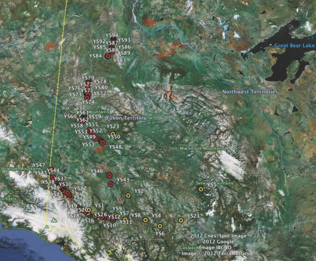
The map below shows the distribution of the 101 sampling sites in the Yukon. We sampled the streams and rivers that traverse the major highways and roads of the Yukon. Sites were sampled upstream of the road. We focused on getting as large a latitudinal gradient as possible to determine how far north D. geminata has spread. The red dots are the sites where D. geminata was not found and the yellow dots are where D. geminata was found.
It should be noted that each site essentially has an equal chance of getting invaded by D. geminata due to the proximity and accessibility of each stream to the roads and highways (fisherman/boats could easily access each site). When looking at the distribution of the sites with and without D. geminata, it can be seen that in some areas a site with D. geminata present is in very close proximity to a site without it, thus suggesting that sites where D. geminata is absent really means that the invasive species cannot handle that particular habitat.
It should be noted that each site essentially has an equal chance of getting invaded by D. geminata due to the proximity and accessibility of each stream to the roads and highways (fisherman/boats could easily access each site). When looking at the distribution of the sites with and without D. geminata, it can be seen that in some areas a site with D. geminata present is in very close proximity to a site without it, thus suggesting that sites where D. geminata is absent really means that the invasive species cannot handle that particular habitat.
Sampling Methods
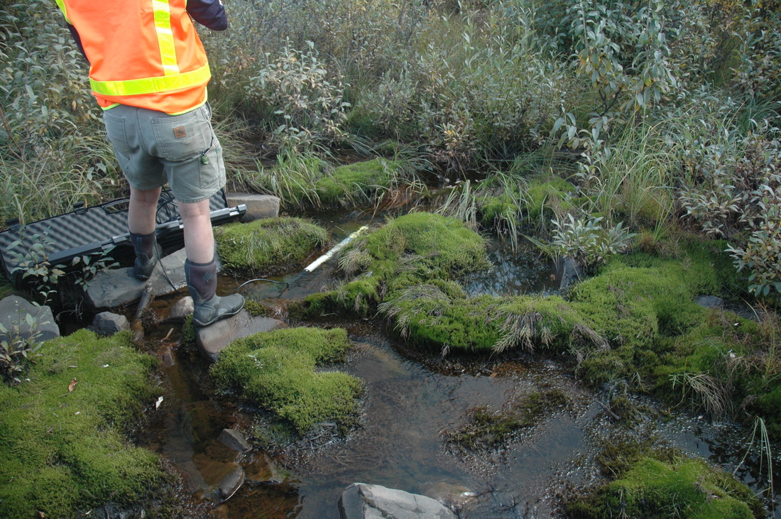
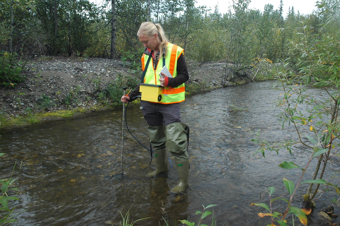
Each stream was examined visually for the presence of D. geminata. Water chemistry variables (pH, conductivity and temperature) was measured with a Hydrolab meter (Figure 5); water velocity of the stream was taken using a current meter (Figure 6) in areas of varying velocities in order to measure an average. Width was estimated for smaller streams and a laser distance meter was used for larger ones.
|
|
|
Figure 5: Hydrolab (white tube) measuring water chemistry of streams. It is placed in a spot where it is submerged in order to minimize atmospheric influence on the measurements.
|
Figure 6: Measuring the current of a stream using a current meter. The meter is pointed upstream.
|
Statistical Analysis
Exploratory graphics were run on the data using the R statistical program. Histograms of each of the environmental factors (Figure 7 in "Results" tab) were done in order to test assumptions, and transformations were used if necessary.
A bar chart with the various predictor variables (Figure 8) was done and possible significant differences were observed between streams with D. geminata present and those without. To test if there was in fact a significant difference between "Presence" and "Absence", a series of two-tailed t-tests were run with a Bonferroni Correction, to take into account the multiple comparisons. The table summarizing the results of the t-tests can be seen in the Results section (Table 2).
A logistic regression was also run on the data in order to determine the relationship between the categorical dependent variables (presence and absence of D. geminata) and the continuous independent variables (pH, conductivity, width, velocity, temperature). A logistic regression is able to work with categorical data by converting them to probability scores and then doing a regression against the continuous independent variables. A table summarizing the results from this analysis can be seen in the Results section (Table 3). It should also be noted that a Bonferroni Correction was also applied to the alpha level which was used in the logistic regression analysis.
Density plots of the raw data (Figure 9) were created in order to determine what ranges of measurements D. geminata preferred if there was any environmental factors that were significantly different between the two dependent variables. Though due to complicated nature of the data, these ranges were determined qualitatively.
